
|
|
Multipotentialmike |
 About and contact
|
Key takeaways
- Poker is a noisy, random game in the short term. A large, unrealistic volume of data is usually required to reach the "long term" and make sensible predictions.
- Fully 97% or more of this variance can be denoised using basic approaches.
- This could be used to evaluate poker-playing bots or general game-play, assist individual players to improve, or develop artificially intelligent coaching apps.
- Machine learning on the player field may be useful in poker room security, or developing players' exploitative gameplay.
The problem
Performance in poker, particularly in online poker, is often measured in terms of the winrate, measured in big blinds won per 100 hands (BB/100), particularly in the cash game format (as compared with tournament-style play).
Depending on the number of players and stake level, winrates vary anywhere from around -25 BB/100 to up to 10-20+ BB/100.
However, random elements in poker mean that a very large number of hands are required to assess a player's true performance. At a typical standard deviation, or "variance", of 70-100 BB/100, we would need over 2 million hands in order to say that a winrate of 1 BB/100 was statistically significant.
Considering that live poker is played at the rate of around 20-40 hands per hour, and online poker in the range of 200-1,000 hands per hour, it would take a significant amount of time to acquire a useful sample, and the oldest hands would fade in relevance by the time we did.
Having a good winrate estimate not only allows the effect of changes in strategy to be feasibly measured, but also the performance of artificially intelligent poker bots to be judged (see Burch et al, 2018, AIVAT paper).
Can we develop machine learning heuristics to obtain a better winrate estimate with a smaller number of hands, and eliminate this bias-recency tradeoff?
The data
I acquired the hand histories for over 150k hands played on PokerStars at NL2 Zoom (stakes of $0.01/$0.02) and wrote a parser to extract board cards, hole cards, and game action for each hand, and performed record linkage on summary data for each hand obtained from the PokerTracker 4 tracking app.
In this game, after each hand is folded, a new one is dealt with no wait time. At any given time, between 300-500 players are playing in this pool. The overall player pool size is on the order of 10,000 over these hands, composed of roughly 2,000 regular players and 8,000 casual or infrequent players.
For each player, PT4 also provides roughly 300 statistics on playing style over the hands we've observed them play in, and this forms an auxilliary database.
Developing approaches
Key concepts: stratificationConsider first of all that instead of poker we have a simple coin-toss game. We have tossed the coin 10 times and won $14. We would therefore estimate that on average we win $1.40 per coin toss.
From the data, the standard deviation is $1.26, so we would estimate that our true winrate is anywhere between $0.62 and $2.18 per cointoss.
Suppose however that we look into the specifics of what happened. Say that our 10 cointosses were made up of 2 tails, for each of which we lost $1, and 8 heads, for each of which we won $2.
It may not be unfair to infer that we lose $1 on every tails and win $2 on every heads. We know that the theoretical frequency of each outcome is 50%, so it looks like we have simply been lucky on this run, having 3 more heads than expected and 3 fewer tails.
If we compute a new estimate with this in mind, the mean becomes: a winrate of 50% x (-1 + 2) = $0.50 per cointoss. Because the within-groups payouts are constant, the variance on them is (separately) zero, so there is no variance in this estimate. It is exact (i.e. we have denoised 100% of the variance). Notice as well that without considering the specifics our original estimate of $1.40 was far off, and even the range did not include the true value. We may well have needed 100 more tosses to get close to the real value.
In poker, we can stratify by different positions (having strong cards, a strong seat in the game, being against weak opponents) in this way to tighten the estimate. It is not that the within-groups variance is zero in this case, however, only that it is lower than the overall average, so we can remove variance with reference to the theoretical frequencies.
Key concepts: all-in equityIn poker, certain situations arise when there is no more strategic play left, and the pot is allocated randomly according to the runout of the cards on the board, after all the players are all-in.
Say that the pot is $100, and we have a 70% chance to win it, and the other player has a 30% chance. The full $100 will go to either us or the other player (Villain in poker jargon), but on average we win 70% x $100 = $70. This so-called all-in equity is smoother than the actual raw winrate, may be different to it in the short term, and has a lower variance. This is a mild denoising technique that many regular poker players already use, but it can be improved upon.
The starting cardsIn a game of Texas Hold'em poker, you are dealt two private cards, called hole cards. Some of these are better than others. Observe the following matrix due to retired actuarial protégé and poker player David Sklansky:
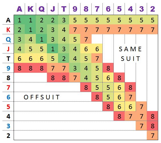
Note that green represents a better hand and red represents a worse hand. Uncoloured hands are quite bad, and are not worth playing, except in specific spots. On the diagonal are pairs, which each occur every 6 in 1,326 hands, on the upper right are suited combinations, occuring every 4 in 1,326, which are slightly better than unpaired combos in the lower left, occuring every 12 in 1,326 hands, since they can form flushes.
The best hand is obviously AA (pocket aces) since no hand can beat this before community cards are dealt.
These 13 x 13 = 169 distinct types of hands already form 169 separate groups on which we can stratify as outlined above to generate two smooth estimates: Heuristic Incomplete Outcome Stratification (HIOS) on the raw winrate (HIOS-Start Raw BB/100) and on the all-in adjusted winrate (HIOS-Start Equity BB/100).
The flopIf we see the first three community cards, called the flop, we have more accurate information to predict how strong our final hand will be and are better able to explain the variance in the final payoff of the hand.
The following diagram illustrates the situation and the remaining two cards to come. In this case we have a set of three aces, a very strong position, and indeed, an unbeatable one here.
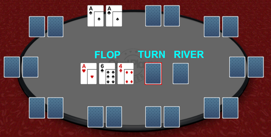
We now have a full hand, and there are 10 different types of hands we may have by here, all of different strengths. The key point is that strong hands should be expected to more consistently win, with lower variance than the overall, and weaker hands should be expected to lose, again more consistently.
For each of the 169 starting combinations, we can further stratify by the following 17 flop outcomes:
| Stratum | Class |
| 1 | High card - no draw |
| 2 | High card - straight draw |
| 3 | High card - flush draw |
| 4 | High card - straight/flush draw |
| 5 | Pair - no draw |
| 6 | Pair - straight draw |
| 7 | Pair - flush draw |
| 8 | Pair - straight/flush draw |
| 9 | Three of a kind |
| 10 | Straight |
| 11 | Flush |
| 12 | Full House |
| 13 | Four of a Kind |
| 14 | Straight Flush |
| 15 | Royal Flush |
| 16 | All-in preflop |
| 17 | Hand ends preflop |
Unfortunately, for the last two strata, we cannot compute the theoretical probabilities because they depend on player behaviour. We can however, average the empirical frequencies for a rough estimate (hence the heuristic).
We therefore have the following matrix of frequencies by starting cards, representing the theoretical breakdown of the 19,600 distinct flop outcomes evaluated by full combinatorial enumeration in C++:
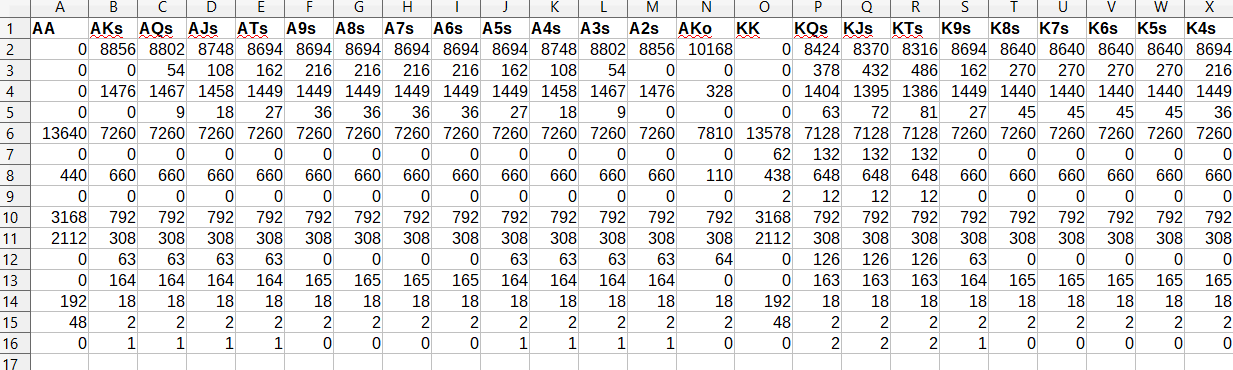
(Note only the first few columns are depicted. AKs is Ace-King suited; AKo is Ace-King offsuited).
Alternative, we could chose to represent this canonical flop outcome matrix (CFO-Mat) in the form of a three-dimensional tensor with the 169 hole cards matrix in the first two dimensions and flop outcome on the third, but for ease I stuck wich a 169 x 16 matrix.
Similarly to before, we now have two additional consistent, unbiased winrate estimators: HIOS-Flop Raw and HIOS-Flop equity.
We could add further stratification dimensions according to position at the poker table, of which there are usually six, and/or the turn and river cards, but if we do so we have far more strata than the number of hands we are sampling from (usually on the order of 20,000) meaning that the model is overdetermined. Each situation is unique, and if we attempt to generalise from each individually we will have either 0 or only 1 hand in each group, so the variance would be theoretically 0, which is obviously incorrect and overly optimistic. Unless there is an intelligent way to group similar outcomes in such a scenario, we stop at the flop.
One other way to handle the flop is rather than using categorical stratification like this, we could regress payoff on equity vs a random two cards conditional on the flop, and convolve this against the theoretical equity distribution, but this is computationally more expensive, and offers less insight for generalisability to improving one's own game.
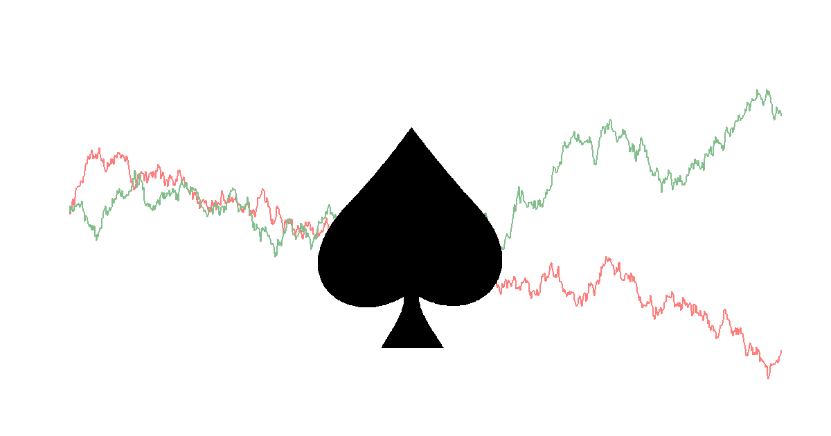
Gaussian ordinary least squares (OLS)The final approach we will consider in mitigating the variance is that of Gaussian OLS. We are all familiar with the idea of drawing a best-fit line through a set of randomly plotted points. It looks like this:
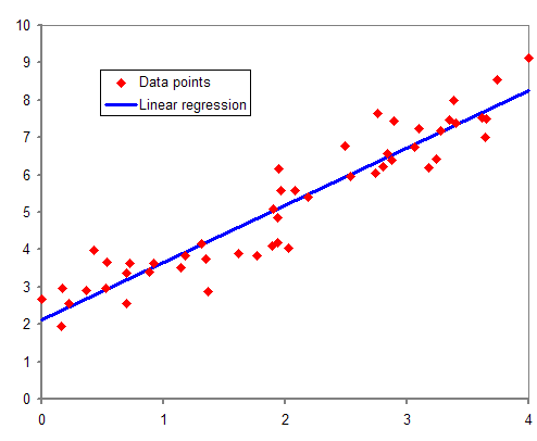
Image credit: Wikimedia Commons
We can do this with either the cumulative winnings or losses according to the raw BB or the equity BB. This has the advantage of not being overly sensitive to large swings (c.f. Cook's distance, and leverage), thus removing variance as we require. Unfortunately, this does not have a sensible intrinsic measure of variance attached like the other methods. The confidence interval on the slope parameter is ridiculously low, because we are working with something like 20,000 hands.
Another thing to bear in mind is that Gaussian OLS requires an assumption of Gaussian or normally distributed residuals, which we do not have here since poker hand payoffs are pathologically platykurtic, i.e. with far heavier tails than the bell curve, similarly to financial returns. I suspect they may even be Cauchy, a famously ill-conditioned distribution.
There may be some ways to rectify this, by the use of trimmed means, removing the most extreme hands in either direction from consideration or by using iteratively reweighted least squares (IRLS), but anyway we have a further two estimators for our true winrate: Gaussian BB and Gaussian equity.
Performance of the estimatorsNow that we have our full set of 8 estimators, let's recall what they are:
| Sample | Raw BB/100 | Equity BB/100 |
| Unstratified | 1 | 2 |
| Gaussian OLS | 3 | 4 |
| HIOS-Start | 5 | 6 |
| HIOS-Flop | 7 | 8 |
And what are the figures when we apply them to our 150k hands?
|
Winrate
|
Variance
|
Notice first of all that our raw variance, 97.2 is exactly in the range we expected from the nature of the game (70-100 BB/100), that the equity approach reduces it somewhat, by about 10-20% for each approach, even the basic, unstratified one. As I mentioned, the Gaussian OLS is artificially small and not very meaningful. However, the HIOS-Flop variance is very small, and believable, around 2.5 BB/100.
In other words, HIOS-Flop is able to remove fully 97% of the variance in poker without too much of a compromise in terms of overfit. In practice, though, it is not quite stable enough to be used in isolation, so we will bring it together with the other metrics:
Introducing CENTREWIRE-LOWESSI recorded the position of the eight indicators on each of roughly 60 consecutive days and plotted the time (in UNIX epoch seconds) against each indicator's measurement. I did this once for the subsample of cumulative hands up until that time, and once for a rolling last 30-days sample.
The key idea is that since all indicators are consistent and unbiased, i.e. with an infinite number of hands they would all be exactly equal and with variance 0, we can take a consensus of what they are pointing to at any given time and expect to be better off than believing any single one alone, since swings in one will be compensated by swings in the other direction in the other.
We can introduce the locally weighted scatterplot smoothing (LOWESS) metric to generate a smooth curve through the points to obtain this consensus at any given time, and I call this the CENTral REgression WInRate Estimate (CENTREWIRE). I also experimented with cubic spline interpolation but it was a little too rugged for the purposes of this project.
The results of this are plotted below:
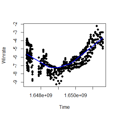
Cumulative |
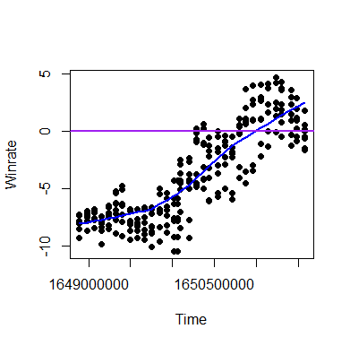
Rolling 30-day |
It is important to note that while we can indeed treat a rolling 30-day period like this, an unequal number of hands are played per day, approximately 2,000 over this period, so a sample size of 60,000 for the 30-day average. This means that the estimates are heteroskedastic, i.e. more tightly spread for 30-day periods for which we have more hands than those for which we don't.
Essentially, however, we are able to generate stable, reliable estimates from a comparatively small volume of data, removing a lot of the variance and significantly mitigating the bias-recency tradeoff.
What we might also have done is an ARIMA time-series decomposition of the original returns (with or without polynomial preserving filter), or applied an indicator like the MESA Adaptive Moving Average (MAMA) to these data, a technical indicator usually employed in financial trading strategies, and known for its ability to more rapidly respond to new data than naïve moving averages.
Other considerations
Sparse regression on the hole cards matrix
In the above stratification approaches, we considered mostly the incomplete outcomes on the flop. If we rewind to the hole cards (or Start) stage, we have a set of 169 hole card combinations, each with their own winrate, or (EV). It stands to reason, and is substantiated in practice, that these winrates are correlated with the quality of these hands, measured in terms of their equity against random combinations of cards (equity, as defined before, is the probability of the cards winning the hand (equity of 100%) or drawing (50% against one Villain).
We may construct a data frame consisting of 5 columns, which are the equity against 1, 2, 3, 4 or 5 villains with random hole cards for each of the 169 canonical starting positions. These are obtained by Monte Carlo simulation in C++.
We then subject these columns to polynomial basis expansion in Matlab, which handles such large matrices gracefully. The key idea in basis expansion is to compute powers and inner products of the columns up to a certain combined sum of the exponents to capture multivariate nonlinear effects, and this appears to work well for poker simulation. An order-32 basis expansion on these data expands our initial 5 columns to 435,897 columns
We can import the resulting model matrix in R using the suitable .mat parsing libraries and use glmnet to conduct a least absolute shrinkage and selection operator (Lasso) regression with these win probabilities reflecting the hand strength as our predictor and the winrate, or EV as our predicted variable.
The Lasso is a very useful tool in selecting from a vast number of irrelevant features those which explain the model best, and does so by introducing a punishment (regularisation parameter lambda) on any variable which is attempting to contribute to the model, to ensure that only the best are selected.
It is also a technique of peculiar interest to me: in my undergraduate group project I developed with my partner an implementation in R of an algorithm already devised by Li, Sun and Toh, and we obtained better objective values using this Semismooth Newton Augmented Lagrangian (SSNAL) method than the industry-standard glmnet, which uses cyclical coordinate descent. The GitHub repository is here.
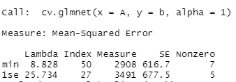
To implement this in practice, we perform a ten-fold cross-validation, training the prediction model on 150 of the combos and seeing how well it does on the other 19. This is done ten times, and the penalisation parameter which minimises the prediction error is obtained.
We then move one standard deviation up from this, since in practice Lasso tends to underpenalise and recover too much of the original model (overfit).
Training diagnostics were as follows:
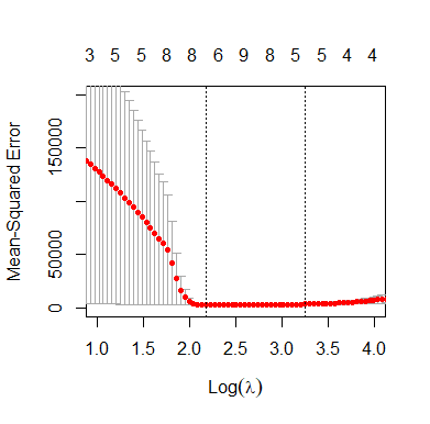
A plot of the predicted against the actual winrate for each combo is given below:
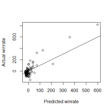
Obviously, the best hand AA, is visible in the upper right, closely followed by KK, the second best hand. It is very reassuring to drill down into the predictions made by the model and see that the worst predicted hand is 72o, which domain-specific player wisdom tells us is indeed the worst hand. Not only that, but the predicted winrate for this hand is around -26 BB/100, which is extremely close to the theoretical maximal loss rate of 25 BB/100 for a 6-max game (folding every hand), and it obtained this value without having been prejudiced towards it with an intercept.
A commonly implemented generalisation of the Lasso is the elastic net regression which interpolates between the Lasso and the ridge, which uses a different penalisation scheme, and on which hyperparameter optimisation can be conducted for the best predictive accuracy.
However, in this case, elastic net regression did not do well, achieving a worse mean-squared error and also didn't pass the sanity check of pushing 72o to the bottom of the prediction pile.
There are two happy consequences of this kind of modelling. Firstly, we can convolve the predicted values for the hands against their theoretical frequencies and obtain yet another stratified winrate estimator. Secondly, we can actually inspect the residuals (that is, the difference between the predicted winrate of a hand given its strength and the winrate achieved in practice) to yield valuable information about the quality of one's personal play.
The worst two residuals in the full model were KJo and AJo, which were fully 113 BB/100 and 173 BB/100 below where we would have expected them to have been. This implies there is something wrong with the way I have been playing them and this is true. I have since polished my game in those two positions.
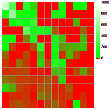
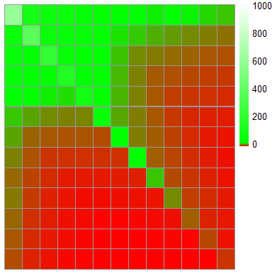
The most striking demonstration of this technique in action is to look at what it does to the heatmap of the hand combinations' winrates, oriented in the same way as the Sklansky matrix above:
|
|
| Actual
winrates by hand. Messy, chaotic, disordered, but clear strength in AA and KK |
Predicted winrates by hand. Smooth, graduated, more sensible theoretically |
The effect of the stack size
Something else to bear in mind when stratifying to produce a winrate estimate is the stack size. For non-poker players, that is the number of chips you have in front of you, relative to the stake level of the game, again measured in big blinds.
To have 80-100 BB is typical. Over 200 is considered deep-stacked and under 80 is considered short-stacked.
The winrate also depends on the stack size. Larger stack sizes usually correspond to higher winrates, particularly for good, winning players. Not only can we construct a multivariate regression on the hand payout using time as a continuous variable, starting cards as a categorical or factor variable, but we may also add stack size.
This allows further refinement of the winrate estimator, and also provides feedback to the player, for instance on whether or not their short-stacked or deep-stacked play is in need of improvement.
In constructing these models I've assumed that starting hands operate independently of stack size, which is not true in practice; deep stacks tend to favour small suited connectors in a way that short stacks do not, and relatively penalise bigger hands.
The addition of a time variable allows us to capture some of the temporal trend that the CENTREWIRE-LOWESS estimate does, and if they coincide, this is good evidence.
Learning on the player field
"Poker is not a game of cards played with people, it is a
game of people played with cards."
Tom McEvoy, WSOP Champion
One final consideration to bear in mind is the composition of the field of players which you are playing against. As an auxilliary data set, I mentioned that PT4 provides 300 variables representing the nature of play for in this case a field of over 10,000 players. Nevertheless, with only 150k hands for our own play, and so many players, we would have on average only 75 (since there are 5 Villains per hand, 15 x 5 = 75) hands per player, though the distribution is Paretian (think 80/20% principle), so there are some for which we have an extraordinary number of hands.
Many of these variables, such as the voluntarily put in pot (VPIP) are percentages and are thus supported on the interval [0,1]. This is a gift to a data scientist, since the data are already standardised and can thus be subjected to multidimensional scaling, which would allow us to apply unsupervised learning mechanisms like agglomorative clustering or the DBSCAN algorithm on these to identify groups of players who play similarly.
I suspect if we did so we would be able to pick out clusters of players which reflect categories already known to those who are familiar with the game, such as LAGs, TAGs, A-Fish, nits, maniacs, recs/regs.
Similarly, we could adopt a supervised approach if we had a gold standard classification, from players with a lot of experience with the field.
These approaches are very useful in a number of ways. Not only could we further refine the winrate estimates and variance denoising techniques if we knew the appropriate proportions of these players in each hand to convolve it against, but we could keep track on how the received wisdom in playing the game evolves and identify new groups of players and playing styles as they arise.
It may also be useful for poker room operators in identifying fraudulent play and account sharing, similarly to how stylometry is used for authorship attribution in forensic linguistics.
It affords the individual player a quick classification method for an unknown (or relatively unknown) villain.
Similarly, continuous or regression-based approaches would prove very valuable in the full assessment of a player field. However, the first thing to note is that player data are very sparse. With few hands on many players, and a variety of comparatively rare spots, a lot of these statistics are simply missing or NA. This is further confused by the fact that as a game of imperfect information, in which Villain makes a choice on whether or not to give you information directly dependent on their cards and position, the data are missing not at random (MNAR) which is the worst form of missingness from which to make inference (missing at random (MAR)/missing completely at random (MCAR) are our best options here).
Logistic regression models on the missingness indicator for each statistic (0 for missing, 1 for present) against number of hands reveal the following general pattern of how many hands we need to have on a player in order to have a 95% chance of having a value for each statistic.
| Statistic | Hands needed |
| BB/100 | 0 |
| Standard deviation (BB/100) | 0 |
| VPIP | 0.82 |
| Attempt to Steal | 9.66 |
| Fold to Steal | 22 |
| Call River Bet | 127 |
| . . . | . . . . |
| Donk/Fold Turn | 3,118 |
| Call Turn 4Bet | 4,506 |
| Fold to River 4Bet | 4,582 |
As you can see, basic statistics like the winrate and standard deviation are maintained on everyone (default value of 0) and very common scenarios like the VPIP require very few hands on a player (in fact, the only time when you would not have a value for this statistic is if the player was on the big blind and everyone else in the hand folded without doing anything).
Similarly, more complex rare situations like Turn and River 4betting (a 4 bet is rare even pre-flop, and many hands do not even reach it to the very last street) require an extraordinary number of hands for what is at that point going to be anyway poor data, subject to extreme variance.
For these missing values, what can be done is stochastic regression imputation or perhaps more appropriately for such complex data as these, predictive mean matching (PMM) or hot-deck imputation.
What may prove to be incredibly useful is to use the set of 300 variable, with or without appropriate imputation for missingness, to predict for a given player on whom one has a small number of hands what the values of those statistics would be when one acquires a larger number of hands, with minimal mean-squared error.
To implement this in practice, it is possible to take the players for whom you have the most hands, partition them down into randomly selected subsamples of hands and use these as training data, with the small subsets as the predictor and the large set as the "gold standard", although necessarily it will itself be subject to some variance. Deming regression has been applied to poker to account for this (see here).
If this achieved accurate estimates on players, it would constitute a substantive edge for the player who managed to do so, without trading in illicit hand histories, rightly prohibited by many poker rooms' TOS since it affords players an unfair edge.
Nevertheless, any studies on the player field would benefit exploitative play, a different playing style to game-theoretically optimal (GTO) play, which is a matter of some debate among poker players. The key difference is that exploitative play looks for weaknesses in the particular opponent, but is itself exploitable, whereas GTO play seeks to develop a strategy which is not exploitable by any other, and is blissfully ignorant of Villain's style. I personally counsel for exploitative play since if everyone in the world were to be playing GTO poker (a stereotypical example of a Prisoner's Dilemma), the winrate distribution would be forced to the Dirac delta distribution, i.e. everyone would win at exactly the same rate: zero.
See also
 |  |